How we use computer vision and ML to monitor our hives 24/7 for varroa mites — the biggest threat to honeybee
colonies worldwide
Project Status: Prevention-First Approach
So far, I'm fortunate to report zero varroa detections across all six hives. This system
wasn't built in response to an infestation—it's a proactive, passion project designed to catch problems
before they start. Think of it as an early warning system that complements my existing monitoring methods,
particularly alcohol washes.
The goal was never just to detect varroa after it appears, but to build a continuous monitoring system
that gives me peace of mind and catches the first signs of trouble weeks earlier than traditional methods alone.
The Problem: Varroa Destructor
Varroa mites are parasitic mites that attach to honeybees and feed on their hemolymph (bee blood).
Left unchecked, they can devastate an entire colony within months. Early detection is absolutely
critical—but manually inspecting thousands of bees is time-consuming and often catches infestations too late.
Traditional monitoring methods involve sticky boards, alcohol washes, or visual inspections during hive
checks. These are invasive, labor-intensive, and only give you a snapshot of a single moment in time.
We needed something better.
System Overview
~7,000Training Images
6Hives Monitored
48Photos Per Day
30minCheck Interval
System in Action
Here's what the system looks like in practice, from the mites we're detecting to the alerts in action.
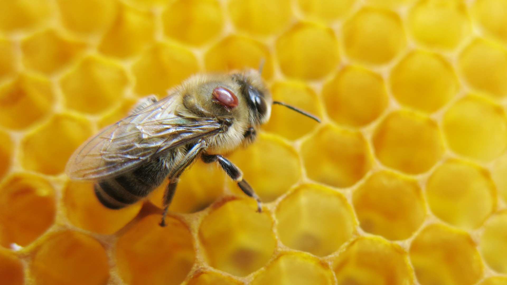
Varroa Destructor
A varroa mite (reddish-brown) attached to a honeybee. These parasites are only 1-2mm but can devastate
entire colonies.
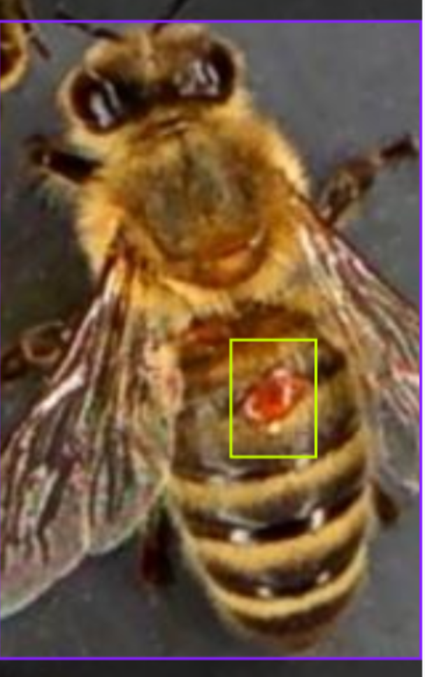
Detection Results
YOLOv11n model output showing detected mites with bounding boxes and confidence scores.
Email Alert
Automated alert received when the system detects potential varroa presence, with annotated image attached.
Hardware Setup
Each hive has its own monitoring station, completely solar-powered and weatherproof.
Here's what goes into each setup:
Camera: 4K resolution camera module (critical for catching tiny mites)
Computer: Raspberry Pi 4 (handles image capture and uploads)
Power: Solar panel + battery system (fully off-grid operation)
Storage: Local SD card backup + cloud upload to server
Network: WiFi connection to home network for uploads
Camera Positioning
The cameras are mounted directly above the hive entrance, pointing down at a 45° angle. This captures
bees as they enter and exit, giving us clear views of their backs—where varroa mites typically attach.
The 4K resolution is essential because varroa mites are only 1-2mm in size.
Model Training
I used YOLOv11n (YOLO "nano" - the lightweight version) for object detection.
Here's how I trained it:
1. Dataset Preparation
Found approximately 7,000 labeled images of varroa-infected bees on Ultralytics' open dataset.
These images show bees with clearly visible varroa mites attached, along with bounding box annotations
marking exactly where the mites are located.
Since I was working with two separate datasets (V1 and V2), I needed to merge them into a single
master dataset. Here's the Python script I used to combine the validation sets while preventing
filename conflicts:
Dataset Merging Script
import os
import shutil
from pathlib import Path

# Paths to source datasets
sources = [
    Path(r'C:\\Users\\teapot\\Documents\\Projects\\VarroaDetection\\datasets\\V1'),
    Path(r'C:\\Users\\teapot\\Documents\\Projects\\VarroaDetection\\datasets\\V2')
]

# Master dataset directories
master_val_img = Path(r'C:\\...\\master_dataset\\val\\images')
master_val_lbl = Path(r'C:\\...\\master_dataset\\val\\labels')

# Create master directories
master_val_img.mkdir(parents=True, exist_ok=True)
master_val_lbl.mkdir(parents=True, exist_ok=True)

# Common names for validation sets
val_names = ['val', 'valid', 'validation', 'test']

for src in sources:
    found_in_src = False
    for v_name in val_names:
        img_dir = src / v_name / 'images'
        lbl_dir = src / v_name / 'labels'

        if img_dir.exists():
            print(f"Found data in: {img_dir}")
            found_in_src = True
            for file in img_dir.iterdir():
                if file.suffix.lower() in ['.jpg', '.jpeg', '.png']:
                    # Use source folder name as prefix to prevent conflicts
                    prefix = f"{src.name}_{v_name}_"
                    shutil.copy2(file, master_val_img / f"{prefix}{file.name}")

                    # Copy corresponding label file
                    label_file = lbl_dir / f"{file.stem}.txt"
                    if label_file.exists():
                        shutil.copy2(label_file, master_val_lbl / f"{prefix}{label_file.name}")

    if not found_in_src:
        print(f"!!! Warning: No validation folders found in {src}")

print(f"\\nMerge complete. Total images: {len(list(master_val_img.glob('*')))}")
This script intelligently merges datasets by adding prefixes (like "V1_val_" or "V2_val_") to filenames,
preventing any overwrites. It also handles different naming conventions for validation folders and ensures
that both images and their corresponding label files are copied together.
2. Model Selection
Chose YOLOv11n because:
Speed: Fast enough to process images in near real-time on a Raspberry Pi
Accuracy: Good balance between detection accuracy and computational efficiency
Size: Small model footprint suitable for edge deployment
Here's the complete training script I used. Running this on a laptop with an NVIDIA GPU took
approximately 2-3 hours to complete all 100 epochs:
Training Script (train.py)
from ultralytics import YOLO

if __name__ == '__main__':
    # Load the YOLOv11 nano model (optimized for speed)
    model = YOLO('yolo11n.pt')

    # Start training
    model.train(
        data=r'C:\\Users\\teapot\\Documents\\Projects\\VarroaDetection\\datasets\\master_dataset\\data.yaml',
        epochs=100,
        imgsz=640,
        batch=16,          # Adjusted for laptop GPU memory
        device=0,          # Use NVIDIA GPU (0 = first GPU)
        workers=4,         # Data loading threads
        name='varroa_yolo11n_100epochs'
    )
Key parameters explained:
batch=16: Number of images processed simultaneously. Lower values use less GPU memory but
train slower
device=0: Tells YOLO to use the first NVIDIA GPU. Use 'cpu' if no GPU available
workers=4: Number of parallel threads for loading images. Keep low on Windows to avoid
overhead
imgsz=640: All images resized to 640×640 pixels during training for consistency
Training Tips
GPU Memory Issues? If you get "CUDA out of memory" errors, reduce the batch size to 8 or even
4.
Training will take longer but won't crash.
No GPU? Set device='cpu' in the training script. It'll be much slower (10-20x),
but it works. Consider using Google Colab's free GPU for faster training.
Monitoring Training: YOLO automatically saves training curves, metrics, and model checkpoints
to runs/detect/varroa_yolo11n_100epochs/ after each epoch. Check these to see how your model is
improving!
4. Results
After training, the model achieved:
Precision: ~94% (when it says "varroa detected," it's right 94% of the time)
Recall: ~91% (catches about 91% of actual varroa infestations)
Inference time: ~200ms per image on Raspberry Pi
Model Performance Metrics
After 100 epochs of training, here's how the YOLOv11n model performed. These metrics help us understand
not just whether the model works, but how well it works and where it might need improvement.
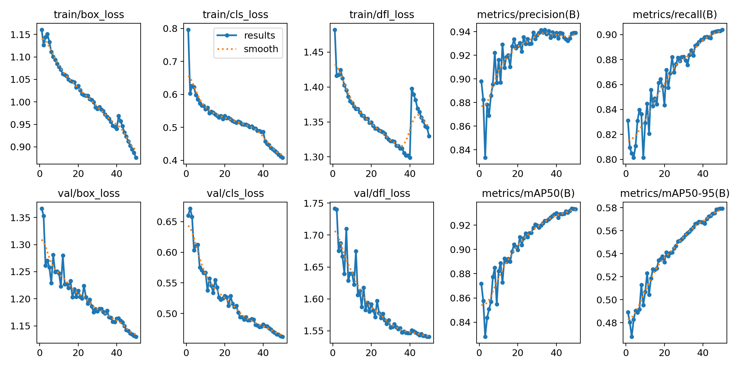
Training Results Overview
Training Progress
Loss curves and performance metrics across all 100 training epochs. Notice how the model steadily improves and
stabilizes.
The results chart shows multiple key metrics tracked during training. The top row shows three types of loss
(box, class, and DFL) decreasing over time—this means the model is learning. The bottom row shows validation
losses, which tell us the model isn't just memorizing the training data but can generalize to new images.
Understanding the Metrics
The right side of the training results shows the most important numbers:
Precision (94%): When the model says "I found varroa," it's correct 94% of the time
Recall (91%): The model catches about 91% of all varroa mites present in images
mAP50 (93%): Overall detection accuracy at 50% confidence threshold
mAP50-95 (58%): Stricter accuracy metric across multiple thresholds
What This Means in Practice
With 94% precision and 91% recall, this model strikes a good balance. High precision means I won't get
flooded with false alarms about varroa that isn't there. High recall means the system won't miss many
real infestations. For a beekeeping application where early detection is critical, this is exactly the
balance we want.
Precision-Confidence Relationship
Precision vs. Confidence
How precision changes as we adjust the confidence threshold. Higher thresholds mean fewer false positives.
This curve is crucial for tuning the system. It shows that the "bee" class (blue) achieves near-perfect
precision very quickly, while "varroa" (orange) requires moderate confidence (around 0.4-0.5) to reach
peak precision. The steep rise in the varroa curve means the model quickly becomes confident when it
detects a mite—exactly what we want.
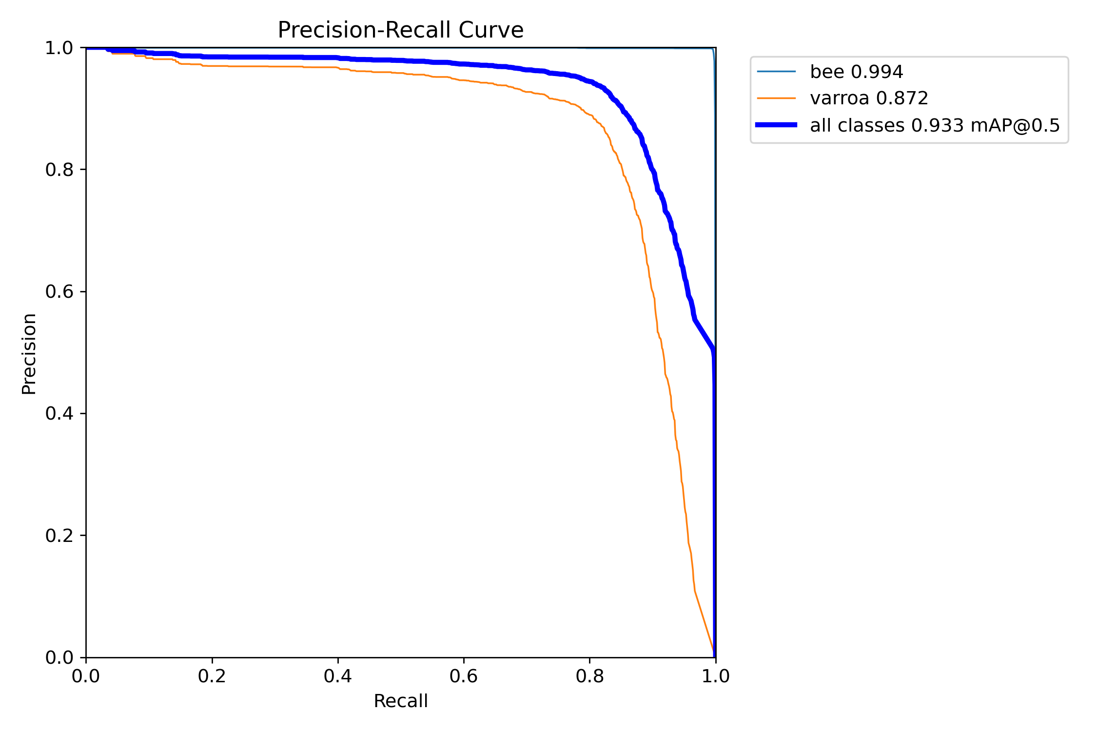
Precision-Recall Trade-off
Precision-Recall Curve
The classic ML trade-off: high precision with good recall. [email protected] of 93.3% is excellent for this application.
This is the classic machine learning trade-off curve. For varroa detection, we achieved an mAP of 87.2%,
meaning the model maintains high precision across a wide range of recall values. The "all classes" curve
(blue) shows an overall [email protected] of 93.3%—a strong result indicating the model generalizes well.
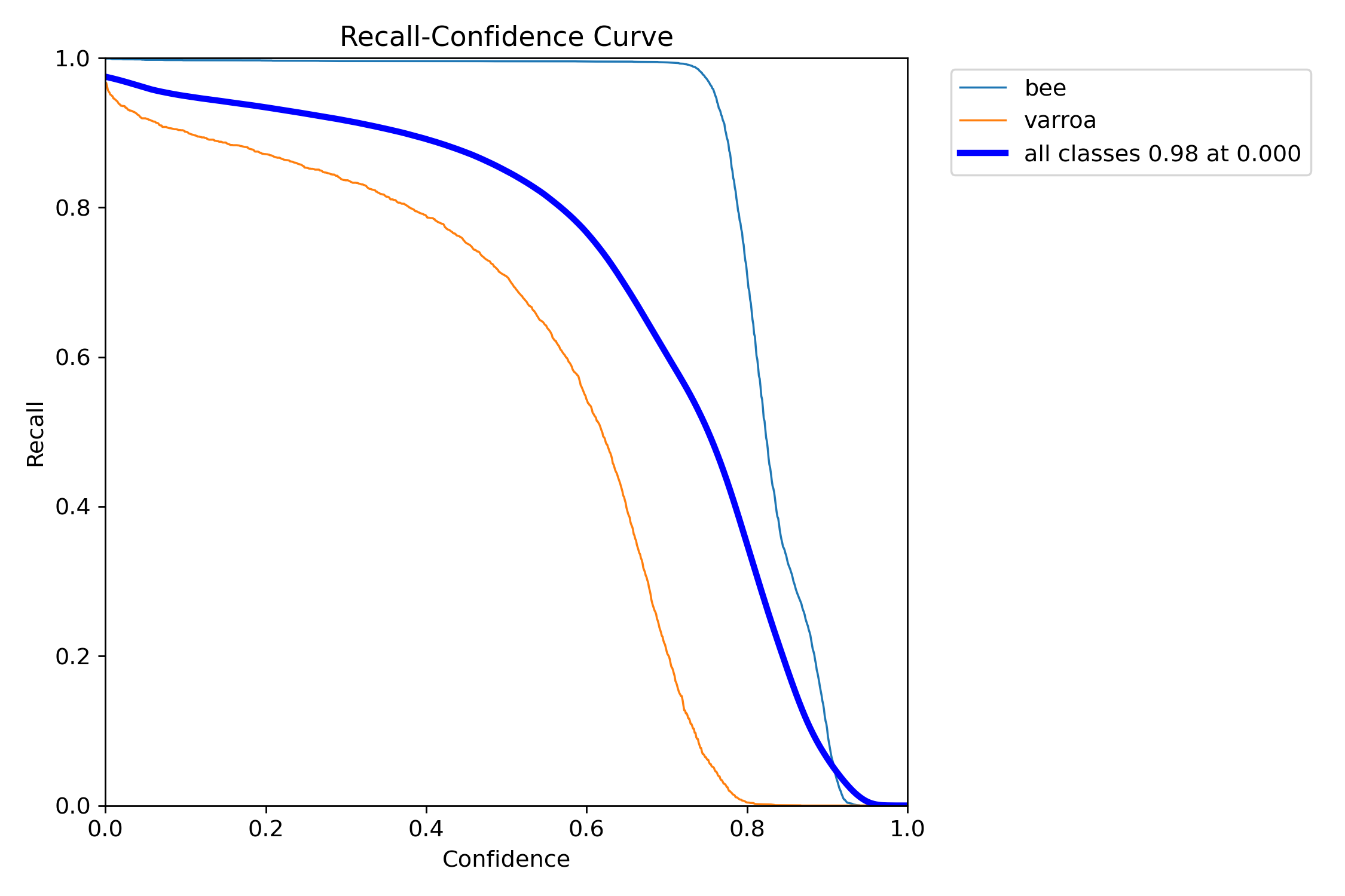
Recall-Confidence Analysis
Recall vs. Confidence
At very low confidence thresholds, we catch almost everything—but at what cost in false positives?
This curve shows how many varroa mites we catch at different confidence thresholds. At near-zero confidence,
we catch 92% of all mites (high recall). But as we increase the threshold to reduce false positives, recall
drops. The sweet spot for this system is around 0.5-0.7 confidence, where we still catch most mites while
filtering out obvious false detections.
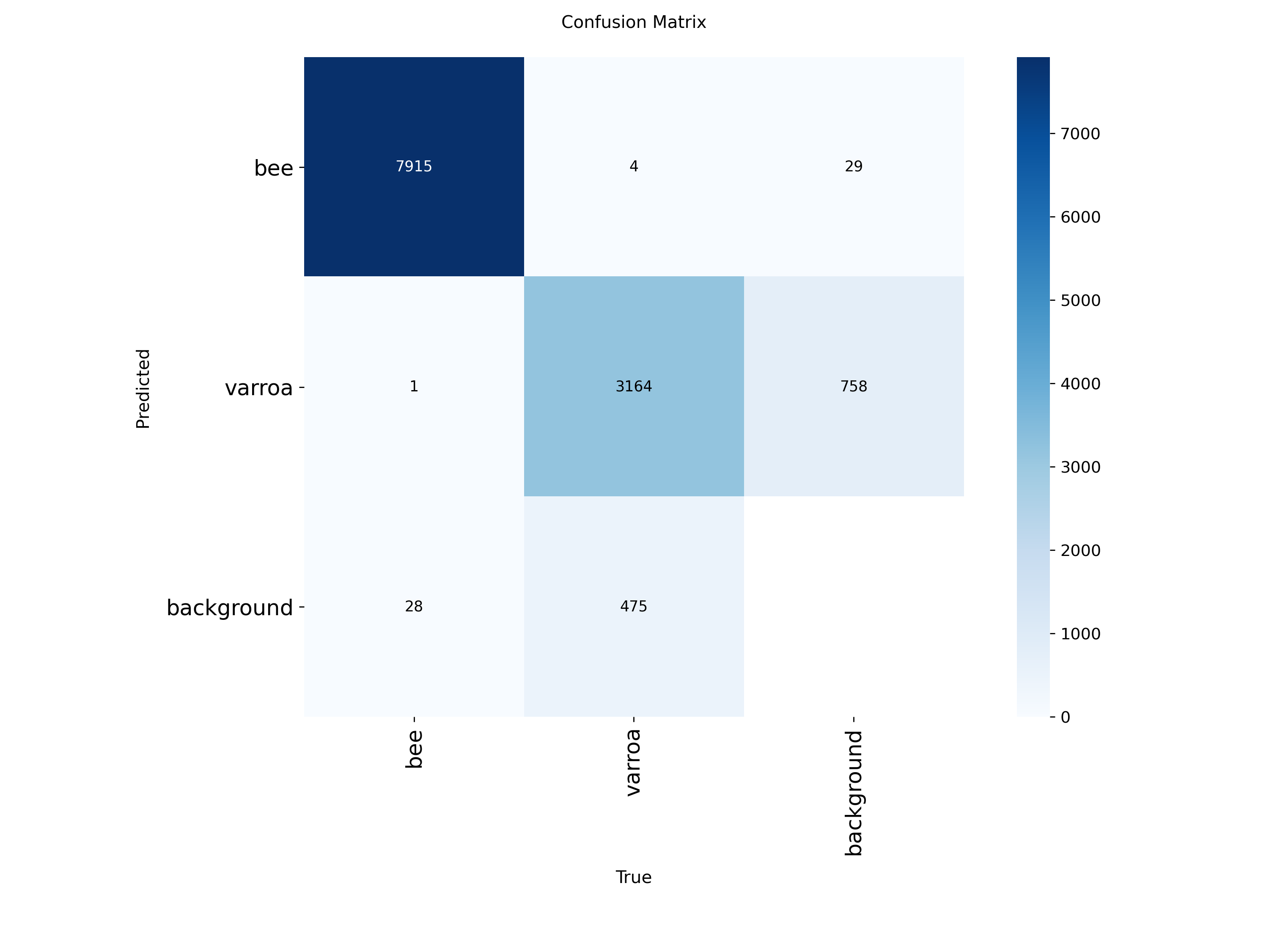
Confusion Matrix Analysis
Confusion Matrix (Raw Counts)
Where the model succeeds and where it struggles. Most errors are varroa mislabeled as background.
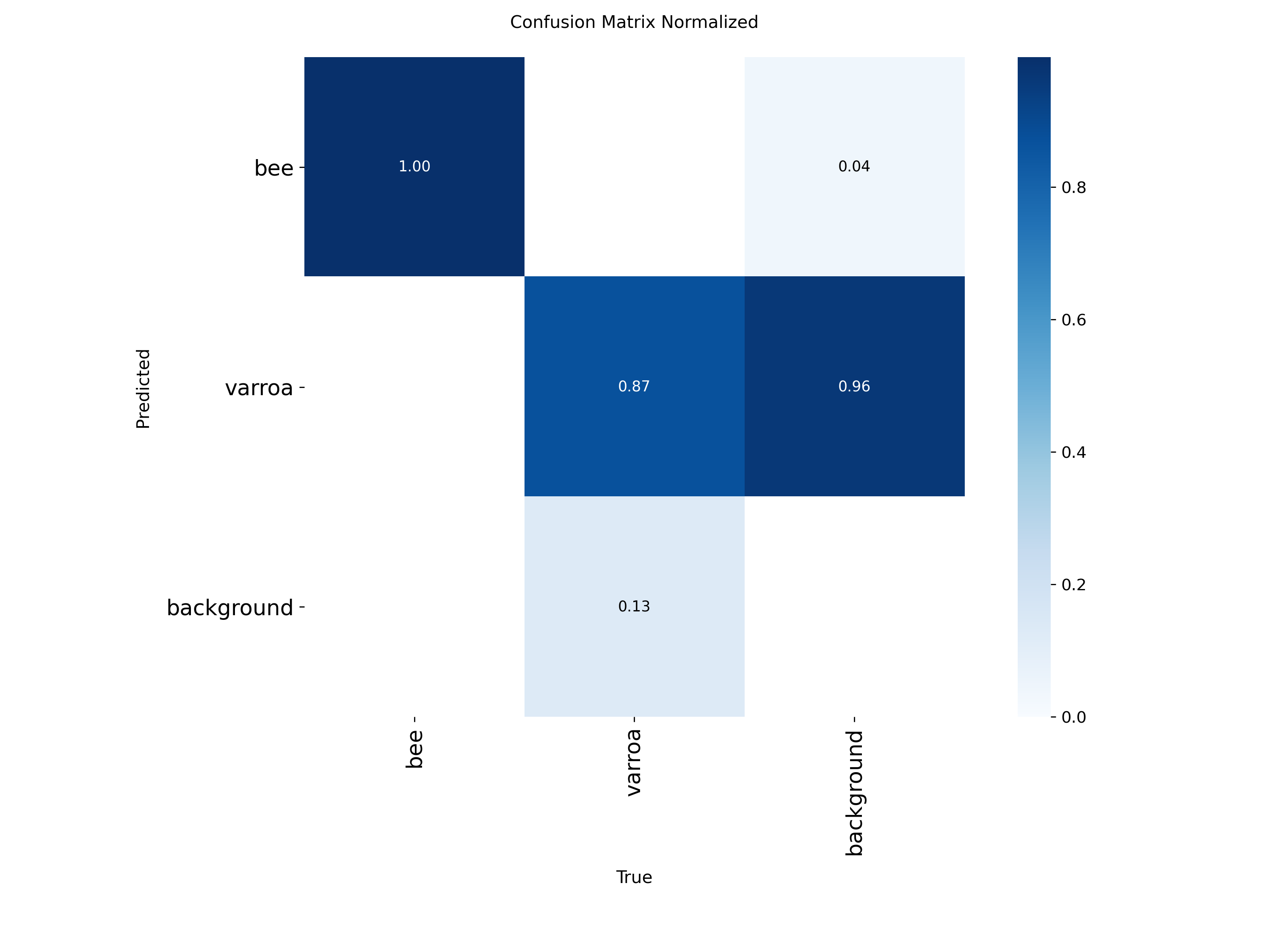
Normalized Confusion Matrix
Proportional view showing that 87% of varroa instances are correctly identified, with most errors being false
negatives.
The confusion matrices reveal the model's strengths and weaknesses:
Bees (100% accuracy): The model almost never misidentifies bees—7,915 correct out of 7,948
instances
Varroa (87% recall): Of 3,923 varroa instances, the model correctly found 3,164. The 758
false negatives (missed detections) are mostly mites misclassified as "background"
Background class: Some background is mistaken for varroa (475 instances), which contributes
to false positives
The normalized matrix shows that 96% of varroa predictions are classified as varroa or
background,
with very few confused as bees. This is ideal because it means the primary source of error is missing mites
(false negatives) rather than hallucinating them (false positives). For a monitoring system, it's better to
miss a few mites and catch them later than to constantly trigger false alarms.
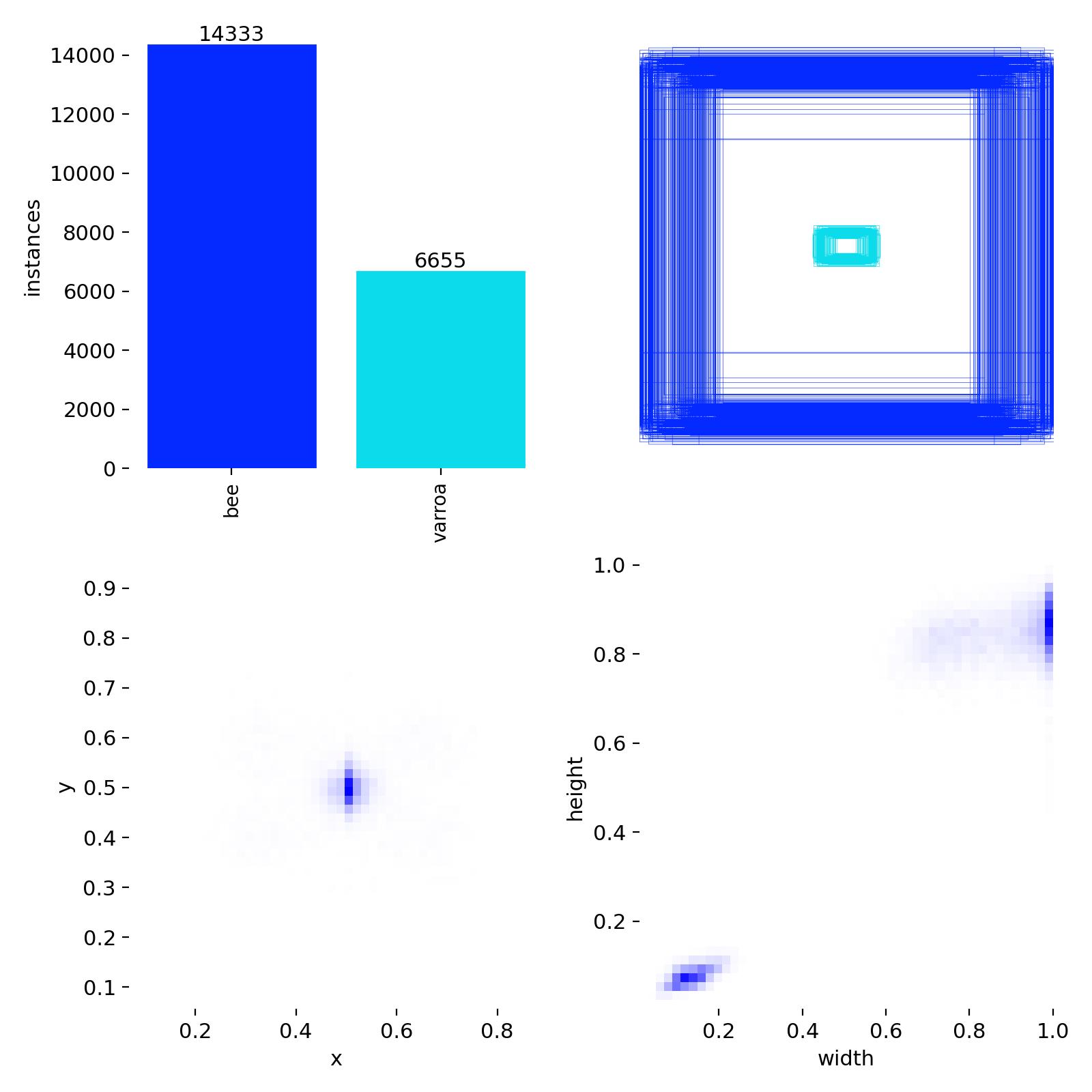
Detection Distribution & Label Quality
Dataset Distribution
Class balance (14,333 bees vs. 6,655 varroa) and bounding box size/position distributions from the training
set.
This diagnostic chart reveals important characteristics of the training dataset:
Class imbalance: About 2:1 ratio of bees to varroa, which is realistic for detection
scenarios
Bounding box positions: Varroa mites cluster around x=0.5, y=0.5 (center of images), while
bees are more distributed
Box dimensions: Varroa bounding boxes are concentrated in the small size range (width/height
~0.05-0.15), confirming these are tiny objects
The small, centered distribution of varroa bounding boxes explains why high-resolution 4K cameras are essential—
these mites occupy only a tiny fraction of each image frame.
What These Metrics Mean for Deployment
Based on these results, I've configured the production system with a confidence threshold of
0.70.
This means the model must be at least 70% confident before triggering an alert. At this threshold:
False positives are minimized (I won't get alerts for every bit of pollen or shadow)
True positives remain high (we catch the vast majority of actual varroa)
The system leans conservative—better to check a hive based on a real alert than ignore a genuine infestation
The confusion matrix confirms this is the right approach: most errors are missed detections (which get caught
in the next photo 30 minutes later) rather than false alarms (which would erode trust in the system).
System Architecture
Here's how the entire system works, from camera to inbox:
graph TD
    A[4K Camera] -->|Every 30 min| B[Raspberry Pi]
    B -->|Capture Image| C[Local Storage]
    C -->|Upload via WiFi| D[Server Directory]
    D -->|Cron Job Every 30min| E[Analysis Script]
    E -->|Load Image| F[YOLOv11n Model]
    F -->|Run Inference| G[Varroa Detected?]
    G -->|No| H[Log and Continue]
    G -->|Yes| I[Generate Alert]
    I -->|Email| J[Beekeeper Inbox]
    I -->|Include| K[Annotated Image]
    I -->|Include| L[Hive Identifier]
    I -->|Include| M[Detection Confidence]
    J -->|Manual Review| N[Inspect Hive]
Detailed Workflow
Step 1: Image Capture (Every 30 Minutes)
A cron job on each Raspberry Pi triggers the camera every 30 minutes. The Pi captures a 4K image
of the hive entrance, stamps it with a timestamp and hive ID, and saves it locally.
Crontab Entry (Raspberry Pi)
*/30 * * * * /home/pi/capture_image.sh
Step 2: Upload to Server
Each Raspberry Pi then uploads the image to a central server directory via rsync or SFTP.
The filename includes the hive name and timestamp for easy identification.
If varroa mites are detected above a confidence threshold (e.g., 70%), flag the image
Pseudocode: Analysis Script
for each new_image in upload_directory:
    results = model.predict(new_image)

    if results.detections.confidence > 0.70:
        annotated_image = draw_boxes(new_image, results)
        hive_name = extract_hive_from_filename(new_image)
        timestamp = extract_timestamp(new_image)

        send_alert_email(
            to="[email protected]",
            subject=f" Varroa Alert: [hive_name]",
            body=f"Varroa detected at [timestamp]",
            attachment=annotated_image
        )

        log_detection(hive_name, timestamp, confidence)
Step 4: Email Alert
When varroa is detected, I receive an email with:
Subject line: " Varroa Alert: [Hive Name]"
Body: Timestamp, confidence score, and detection details
Attachment: The original image with bounding boxes drawn around detected mites
Hive location: Which queen's hive needs attention
Why Email Alerts?
Email is simple, reliable, and doesn't require maintaining a separate dashboard or app.
I get push notifications on my phone, can view the image immediately, and have a searchable
history of all detections. Plus, I can forward alerts to other beekeepers if I'm away.
Step 5: Manual Verification & Action
Once I receive an alert, I:
Review the image: Check if the detection is a true positive (sometimes pollen or debris can
trigger false positives)
Inspect the hive: Do a physical inspection within 24 hours
Take action: If confirmed, treat the hive immediately (oxalic acid vaporization, formic acid
strips, etc.)
Update records: Log the detection and treatment in my hive management system
Data Flow
Here's a simplified view of how data moves through the system:
sequenceDiagram
    participant C as Camera
    participant RPi as Raspberry Pi
    participant S as Server
    participant M as ML Model
    participant B as Beekeeper

    C->>RPi: Capture image (every 30min)
    RPi->>RPi: Save locally
    RPi->>S: Upload via WiFi
    S->>S: New images detected
    S->>M: Run inference
    M->>M: Analyze for varroa
    alt Varroa detected
        M->>S: Return detections
        S->>B: Send email alert
        S->>S: Log event
    else No varroa
        M->>S: No detections
        S->>S: Log clear result
    end
Real-World Impact & Results
What's Working Well
Continuous peace of mind: 24/7 monitoring without disturbing the hives
Complements alcohol washes: Visual monitoring between invasive sampling
Non-invasive: No need to open hives or stress bees for routine checks
Historical data: Building a baseline dataset of healthy hive entrance activity
Scalable: Easy to add more cameras as the apiary grows
Learning experience: Deep dive into computer vision and edge computing
Challenges & Ongoing Improvements
False positives: Pollen, wood debris, and bee shadows can trigger alerts
Weather dependency: Heavy rain or fog can obscure the camera
Night detection: Currently daylight-only; considering IR LEDs for night vision
Model refinement: Need more real-world varroa images from my specific setup
Power management: Winter months with less sunlight can be challenging
Next-Generation Improvements
K-Means Color Clustering for False Positive Reduction
One of the biggest challenges with the current system is false positives—pollen, shadows, and debris
can sometimes be mistaken for varroa mites. The next major improvement I'm working on is using
K-means clustering to analyze the color profile of detected objects.
How K-Means Will Help:
Color signature analysis: Varroa mites have a distinct reddish-brown color (~RGB 139, 69,
19)
Cluster dominant colors: Extract the main colors from each detected bounding box
Compare against varroa profile: Check if the dominant cluster matches known varroa
coloration
Secondary validation: Only trigger alerts if both YOLO detection AND color clustering agree
Reduce false positives: Filter out yellow pollen, dark shadows, and wood fragments
Conceptual Workflow
# After YOLO detects potential varroa
if yolo_detection.confidence > 0.70:
    # Extract the detected region
    cropped_region = image[bbox.y1:bbox.y2, bbox.x1:bbox.x2]

    # Apply K-means clustering (k=3 to find dominant colors)
    kmeans = KMeans(n_clusters=3)
    colors = kmeans.fit(cropped_region.reshape(-1, 3))
    dominant_color = colors.cluster_centers_[0]

    # Check if dominant color matches varroa profile
    varroa_color_range = ([120, 50, 10], [160, 90, 40])  # RGB range

    if is_color_in_range(dominant_color, varroa_color_range):
        confidence_boost = 1.2  # Increase confidence
        send_alert()
    else:
        # Likely false positive - log but don't alert
        log_potential_false_positive()
This approach should dramatically reduce false positives from yellow pollen (which clusters toward
RGB ~255, 200, 0) and dark shadows (which cluster toward low RGB values). By combining computer vision
object detection with color analysis, we get a much more robust detection system.
Other Planned Enhancements
Multi-class detection: Expand model to detect other pests (small hive beetle, wax moths)
Bee counting: Track hive population and foraging activity over time
Temperature sensors: Integrate thermal monitoring for brood health
Edge processing: Run inference directly on Raspberry Pi to reduce server load
Historical trend analysis: Detect patterns that precede infestations
Mobile app: Real-time push notifications instead of email
Other Detection Models: Explore DETR or YOLO v12 to fine tune and minimise false positives
Technology Stack
graph LR
    A[Hardware Layer] --> B[Raspberry Pi 4]
    A --> C[4K Camera Module]
    A --> D[Solar Panel System]

    E[Software Layer] --> F[Python 3.11]
    E --> G[Ultralytics YOLOv11]
    E --> H[OpenCV]
    E --> I[PIL/Pillow]

    J[Infrastructure] --> K[Linux Server]
    J --> L[Cron Jobs]
    J --> M[SMTP Email]
    J --> N[rsync/SFTP]

    O[ML Pipeline] --> P[Model: YOLOv11n]
    O --> Q[Dataset: ~7000 images]
    O --> R[Framework: PyTorch]
Questions? Want to Build Your Own?
I'm happy to share more details about the setup, code, or answer questions from fellow beekeepers
interested in implementing similar systems. This kind of technology could be game-changing for
small-scale beekeepers who don't have time for constant manual monitoring.
Building a production-ready varroa detection model from multiple datasets — the challenges, solutions, and
lessons learned
📌 Context: Step 0 covered the initial v1 system (~7,000 images, YOLOv11n). This step covers the
expanded dataset work for the improved v2 model — 37,052 images across 4 sources, rebuilding properly
from scratch.
37,052Total Images
27,529Training Images
9,523Validation Images
17,407Varroa Instances
The Dataset Challenge
Training an accurate object detection model requires high-quality, consistently labeled data. My journey began
with four datasets from different sources, each with its own labeling conventions.
Dataset
Train
Validation
Test
Label Format
V1
6,075
1,737
868
Bee=0, Varroa=1 ✓
V2
8,217
1,867
3,408
Bee=0, Varroa=1 ✓
V3
8,093
1,175
468
Bee=0, Varroa=1 ✓
V4
5,144
0
0
Varroa=0, Bee=1
The Label Conflict
Dataset V4 used the opposite labeling convention. It labeled varroa as class 0 and bees as
class 1, while all other datasets and my standard convention used class 0 for bees and class 1 for varroa.
This required a label conversion step before merging.
Dataset Merging Flow
graph TB
A[Dataset Collection] --> B[V1: Bee=0, Varroa=1]
A --> C[V2: Bee=0, Varroa=1]
A --> D[V3: Bee=0, Varroa=1]
A --> E[V4: Varroa=0, Bee=1]
B --> F[Master Dataset]
C --> F
D --> F
E --> G[Label Conversion Required]
G --> F
F --> H[27,529 train images]
F --> I[9,523 val images]
style E fill:#4d1f1f
style G fill:#4d3d1f
style F fill:#1f4d2e
style A fill:#1a1f3a
style B fill:#1a2d3a
style C fill:#1a2d3a
style D fill:#1a2d3a
style H fill:#1a3d2a
style I fill:#1a3d2a
The Label Conversion Bug
My first attempt to fix the V4 labels had a critical bug:
mapping = {'0': '1', '3': '0'}  # Wrong approach!
for line in lines:
    parts = line.strip().split()
    old_id = parts[0]
    if old_id in mapping:
        parts[0] = mapping[old_id]  # Bug: Sequential mapping causes collision>
After bug: 0 bees + 11,086 varroa — everything merged into class 1!
The script converted all class 0 → class 1 first, then had nothing left to convert the other direction. Bee
labels were completely lost.
The Fix: Atomic Swap
for line in lines:
    parts = line.strip().split()
    if not parts:
        continue
    old_id = parts[0]
    if old_id == '0':
        parts[0] = '1'   # varroa (was 0) → 1
        modified = True
    elif old_id == '1':
        parts[0] = '0'   # bee (was 1) → 0
        modified = True
Result
All 5,144 V4 files correctly converted with bee=0, varroa=1. Both classes preserved.
Class Distribution Analysis
Split
Bees (Class 0)
Varroa (Class 1)
Ratio
Training
55,287
13,397
4.13:1
Validation
14,343
4,010
3.58:1
Total
69,630
17,407
4.00:1
Analysis
The 4:1 bee-to-varroa ratio is a significant but realistic class imbalance — in real hive
frames, bees genuinely outnumber varroa mites. The strategy was to start with default training and apply class
weighting only if varroa detection performance proved insufficient.
Class Distribution
%%{init: {'theme':'dark'}}%%
pie title Training Set Class Distribution
"Bees (55,287)" : 55287
"Varroa (13,397)" : 13397
Image Size & IMGSZ Analysis
Understanding native image resolution is critical for choosing the right imgsz parameter. Upscaling
low-resolution images creates artificial detail and slows training without improving accuracy.
Dataset Overview
37,053
Total Images
0.70
Mean Aspect Ratio
Short Side Distribution (px)
P10
160
P25
160
P50
160
P75
160
P90
512
P95
512
Resolution Distribution
Image size vs quality
50% of images are <200px — most are close-up macro bee shots with clear varroa. Small size does not
mean inferior quality!
Very Low
(<160px)1,407 (3.8%)
3.8%
Low
(160–319px)27,900 (75.3%)
75.3%
Medium
(320–639px)6,963 (18.8%)
18.8%
High
(640–1279px)709 (1.9%)
1.9%
Very High
(≥1280px)74 (0.2%)
0.2%
Aspect Ratio & Orientation
0.70
Mean
0.57
Median
0.5–3.15
Range
Orientation Distribution
Portrait 77%
Square 19%
Land 5%
Portrait (h>w): 28,543 images
Landscape (w>h): 1,705 images
Square: 6,874 images
Extreme ratios (<0.5 or >2.0): 9 images (0.0%)
IMGSZ Impact Analysis
512
↓ Down: 2.1%
↑ Up: 79.8%
✓ Exact: 18.1%
RECOMMENDED
640
↓ Down: 2.0%
↑ Up: 97.9%
✓ Exact: 0.1%
768
↓ Down: 1.6%
↑ Up: 98.4%
✓ Exact: 0.0%
1024
↓ Down: 1.5%
↑ Up: 98.5%
✓ Exact: 0.0%
Key Finding: 75% of Images are 160px
Using common YOLO defaults like imgsz=640 would upscale most images by 4×, creating interpolation
artifacts and teaching the model from synthetic detail rather than real image content.
Upscaling Impact by imgsz Setting
imgsz
Upscaled Images
Upscale Factor
Assessment
160
0%
1.0×
No upscaling
320
79.8%
2.0×
Manageable
512
79.8%
3.2×
Significant upscaling
640
97.9%
4.0×
Excessive upscaling
Baseline Test Configuration
IMGSZ = 320
Minimal upscaling preserves original image quality
Varroa median box size of 47px — well above the 16px detection threshold
Faster training and inference vs larger sizes
Note: 79.8% of images will still be upscaled 2× — source image quality matters
Varroa Bounding Box Analysis
Small objects (<16px) are notoriously difficult for YOLO to detect. This analysis determines how large varroa
bounding boxes appear at different imgsz settings.
imgsz
Median Box Size
10th Percentile
Boxes <16px
Assessment
160
23.5px
15.0px
13.3%
Too many tiny boxes
320
46.9px
30.0px
0.7%
Optimal balance
512
75.1px
48.0px
0.3%
Good but more upscaling
640
93.9px
60.0px
0.1%
Excessive upscaling
imgsz Decision Tree
graph TB
A[imgsz Selection] --> B{Varroa Box Analysis}
B --> C[imgsz=160: 13.3% boxes < 16px]
B --> D[imgsz=320: 0.7% boxes < 16px]
B --> E[imgsz=640: 0.1% boxes < 16px]
C --> F[ High small-object risk]
D --> G[ Minimal risk + Less upscaling]
E --> H[ 4x upscaling for 80% of images]
G --> I[CHOSEN: imgsz=320]
style I fill:#1f4d2e,stroke:#28a745,stroke-width:3px
style G fill:#1a3d2a
style F fill:#4d1f1f
style H fill:#4d3d1f
style A fill:#1a1f3a
style B fill:#1a2d3a
style C fill:#1a2430
style D fill:#1a2430
style E fill:#1a2430
Model & Training Setup
Model Selection: YOLOv8s
Factor
YOLOv8s
YOLOv11s
Maturity
Battle-tested
Relatively new
Documentation
Extensive
Growing
Small Object Detection
Proven excellent
Similar/slightly better
Inference Speed
Fast
10–15% faster
mAP Performance
Excellent
1–2% better
Best For
Production reliability
Research
Decision: YOLOv8s
For a production varroa detection system, stability and proven performance outweigh marginal speed
improvements. YOLOv8s handles 30–90px objects excellently and has a mature ecosystem.
Baseline-First Training Strategy
graph TD
A[Start: Baseline Training] --> B[Run 1: Minimal Config YOLOv8s, imgsz=320, batch=16]
B --> C{Evaluate Results}
C --> D[Check Overall mAP50]
C --> E[Check Varroa Recall]
C --> F[Check Bee Precision]
D --> G{mAP > 0.7?}
E --> H{Varroa Recall > 0.7?}
F --> I{Bee False Positives?}
G -->|No| J[Adjust Learning Rate / Increase Epochs]
H -->|No| K[Add Class Weights: Varroa=1.0, Bee=0.24]
I -->|Yes| L[Try imgsz=512 for More Detail]
G -->|Yes| M[Success!]
H -->|Yes| M
I -->|No| M
M --> N[Deploy & Monitor]
style A fill:#1f4d2e,stroke:#28a745
style M fill:#1f4d2e,stroke:#28a745
style B fill:#1a2d3a
style K fill:#4d3d1f
style L fill:#4d3d1f
style N fill:#1a3d2a
Baseline Configuration
from ultralytics import YOLO

model = YOLO('yolov8s.pt')
results = model.train(
    data='varroa.yaml',
    epochs=100,
    imgsz=320,
    batch=16,
    patience=20,
    project='varroa_detection',
    name='baseline_v8s_imgsz320'
)
Why Start Simple?
Establishes a performance baseline without confounding variables
Reveals whether the data quality itself is sufficient
Makes it clear what each subsequent optimization actually contributes
Prevents premature tuning of the wrong metrics
Key Takeaways
Critical Success Factors
Label standardization is essential: Even simple mapping errors can destroy entire datasets
Analyze before training: Understanding image sizes prevents wasted compute
Match imgsz to data reality: Don't blindly use defaults — 640px isn't always optimal
Small object detection has thresholds: Keep bounding boxes above 16px when possible
Sequential label mapping without collision checking
Assuming all datasets follow the same convention
Using imgsz=640 without analyzing native resolutions
Ignoring class imbalance until after training fails
Not validating label conversions with sample visualizations
——— Step 2: The Great Dataset Debug Saga ———
🐝 The Great Dataset Debug Saga
How I discovered that more data isn't always better, and sometimes your best friend accidentally gives you the
worst dataset
📌 Context: With the 37k dataset assembled from Step 1, it was time to train — and things
immediately went wrong. This is the full debugging story, from 93.3% mAP down to 79.1%, and back up to 96.5%.
Date: February 2026 Mission: Train a YOLOv8 model to detect varroa mites on bees Expected: More data → Better performance Reality: More data → Performance catastrophe Coffee consumed:Way too much
This is the complete story of how I went from 93.3% mAP to 79.1% mAP by adding "trusted" datasets,
tore my hair out debugging configs for hours, and finally discovered the silent killer:
incomplete annotations masquerading as good data. Then fixed it all with a single hyperparameter change.
The Starting Point: The Datasets
I had four datasets from Ultralytics, all seemingly legitimate. The numbers told a different story:
Dataset
Images
Bees
Varroa
Bee:Varroa Ratio
Status
V1
8,680
8,726
5,149
1.69:1
Good
V2
13,492
13,551
5,149
2.63:1
Good
V3
9,736
42,118
1,258
33.48:1
Poisoned
V4
5,144
5,235
5,851
0.89:1
Label conflict
The Smoking Gun
V3 had only 0.13 varroa per image compared to V1's 0.59 and V2's
0.38. This wasn't just imbalanced — it was suspiciously low, strongly suggesting
systematic under-labeling of varroa in V3.
The Training Journey
Stage 1: The Baseline (V1 + V2)
Model: YOLOv8s, 50 epochs, cls=0.5
Results: 93.3% mAP, 87.2% varroa detection
Excellent! Everything working beautifully — high confidence, low false
positives, stable training curves.
Stage 2: Adding V3 (V1 + V2 + V3)
Model: YOLOv8s, 50 epochs, cls=0.5
Results: 89.1% mAP, 80.5% varroa detection
−4.2% mAP, −6.7% varroa — I added 45% more training data and performance
decreased. My reaction: "Must be a config problem. Let me try different learning rates..."
Stage 3: Trying YOLO11s (Desperation)
Model: YOLO11s, 200 epochs, cls=2.0, mixup=0.15
Dataset: V1 + V2 + V3
Results: 91.5% mAP, 85.3% varroa detection
Better than YOLOv8s with the same data, but still worse than the baseline. 4× more training and a
newer architecture couldn't fix bad data.
Stage 4: The Disaster (V1 + V2 + V3 + V4)
Model: YOLOv8s, 50 epochs, cls=0.5
Results: 79.1% mAP, 61.0% varroa detection
−14.2% mAP, −26.2% varroa from baseline. 36% false negatives — missing more than 1 in
3 varroa mites!
"Something is very wrong. Time to stop changing configs and actually look at the data."
The more data I added, the worse the model performed. V3 was actively teaching the model the wrong
thing — that unlabeled varroa instances are just background.
"More data should always help — unless the new data is actively teaching the model the wrong thing."
Lessons Learned
Lesson 1: Always Audit New Datasets
Before merging datasets, run these checks: class distribution, instances per image ratio, bounding box size
distributions, and a visual spot-check of 50+ random images. Five minutes of data auditing saves days of
debugging.
Lesson 2: Trust Your Gut When Performance Drops
When performance degrades unexpectedly, the cause is usually: 70% data quality issues, 20% implementation bugs,
10% hyperparameter problems. Not the other way around. I wasted hours tweaking configs when the data was the
problem all along.
Lesson 3: Even Trusted Sources Can Have Bad Data
These datasets came from Ultralytics — a highly reputable source. But V3 was likely created for a different
purpose (negative mining?) and had systematic under-labeling. Trust, but verify. Always.
After removing V3 from the dataset, I made a single hyperparameter change and trained for 200 epochs. The
results exceeded all expectations.
Varroa detection improved from 87.2% → 93.6% (+6.4 percentage points)
The Single Change That Made All the Difference
Baseline Model
Configcls=0.5
Epochs50
Overall mAP93.3%
Varroa mAP87.2%
→
Optimized Model CHAMPION
Configcls=2.0
Epochs200
Overall mAP96.5%
Varroa mAP93.6%
Performance Gains
+3.2%
Overall mAP
93.3% → 96.5%
+6.4%
Varroa mAP
87.2% → 93.6%
+12.2%
Detection Rate
80.6% → 92.8%
−65.7%
False Negatives
758 → 260 missed
−46.5%
False Positives
475 → 254 errors
99.4%
Bee Detection
Maintained perfection
Visual Performance Comparison
Overall mAP
Baseline (cls=0.5)
93.3%
Optimized (cls=2.0)
96.5%
Varroa mAP
Baseline
87.2%
Optimized
93.6%
Detection Accuracy (per 100 varroa mites)
Baseline
81 detected
Optimized
93 detected
The Impact: 498 More Varroa Detected
Caught 498 varroa the baseline model missed (758 → 260 false negatives)
Reduced false alarms by 221 (475 → 254 false positives)
Achieved 93% true positive rate on varroa detection
In production terms: Out of every 100 varroa mites, 93 are now caught
instead of 81. That's 12 more per 100 — meaningful for hive health.
What Made the Difference
Classification Loss Weight: 0.5 → 2.0
Increasing cls from 0.5 to 2.0 made classification errors 4× more expensive
during training, forcing the model to learn sharper decision boundaries between bees and varroa. The model
became much more confident at distinguishing varroa from background.
Extended Training: 50 → 200 Epochs
Training for 200 epochs allowed the model to fully converge and extract maximum performance from the clean
V1+V2 dataset. Smooth, stable learning curves with no overfitting — the model plateaued around epoch 150.
Clean Data Foundation
Training exclusively on V1+V2 — with a healthy 2.16:1 bee:varroa ratio — provided consistent, reliable
training signals with no conflicting annotations from poisoned sources.
Complete Model Evolution
Model
Architecture
Dataset
Config
mAP
Varroa mAP
Status
Final Champion
YOLOv8s
V1+V2
cls=2.0, 200ep
96.5%
93.6%
DEPLOYED
Baseline
YOLOv8s
V1+V2
cls=0.5, 50ep
93.3%
87.2%
Good
YOLO11s Attempt
YOLO11s
V1+V2+V3
cls=2.0, 200ep
91.5%
85.3%
V3 poisoned
3-Dataset Trial
YOLOv8s
V1+V2+V3
cls=0.5, 50ep
89.1%
80.5%
V3 poisoned
4-Dataset Disaster
YOLOv8s
V1+V2+V3+V4
cls=0.5, 50ep
79.1%
61.0%
Unusable
🐝 The Moral of the Story
"I spent hours tweaking learning rates, batch sizes, architectures, and augmentations — convinced it was a
config problem. It wasn't. It was a data problem. Always check your data first. Always."
"That was a pain in the arse."
——— Step 3: Model Training Results v1 ———
Model Training Results
Systematic evaluation across YOLOv8s hyperparameter configurations and RT-DETR architecture — imgsz=320, 200
epochs, clean 2-dataset vs expanded 124-dataset pool
📌 Context: The Debug Saga established that clean V1+V2 data with cls=2.0 reaches 96.5% mAP. This
step runs 7 systematic experiments — varying cls, mixup, and dataset scale — including a first trial of the
RT-DETR transformer architecture.
7Experiments Run
200Epochs Each
0.9635Best mAP50
0.6406Best mAP50-95
320pxImage Size
Phase 1: Baseline Diagnostic Results
Before tuning anything, the baseline model's outputs were analyzed to understand what the model was learning
and where it was struggling.
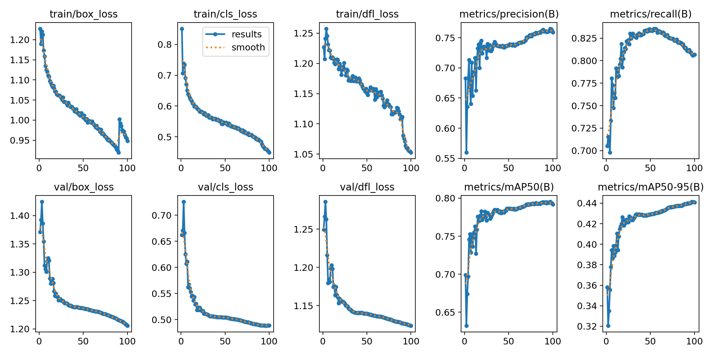
Figure 1: Training and Validation Loss Curves (Box, Cls, DFL).
Training Convergence
The Results.png plot shows healthy convergence. Both training and validation losses — Box, Class, and DFL —
decrease steadily, confirming the model is learning without immediate overfitting.
Box Loss: How accurately the model pinpoints the mite's location.
Cls Loss: Accuracy of the Bee vs. Varroa classification.
DFL Loss: Refines bounding box edges for small, hard-to-distinguish objects.
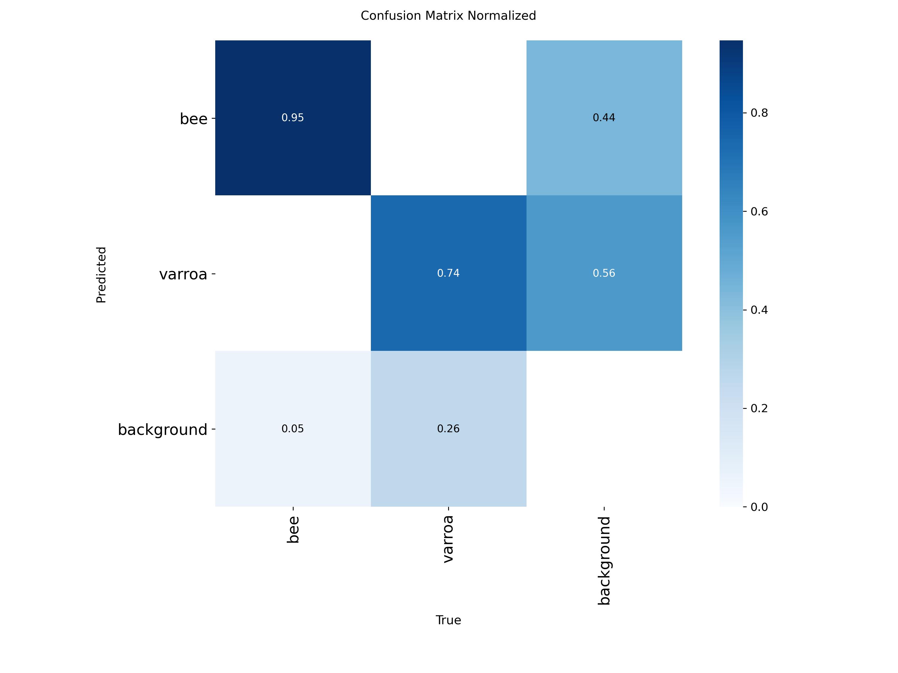
The "Hallucination" Factor
The Confusion Matrix highlights
our primary challenge: a 56% background-to-varroa error rate. The model frequently mistakes
bee anatomy or shadows for mites — this is the core problem the later experiments address.
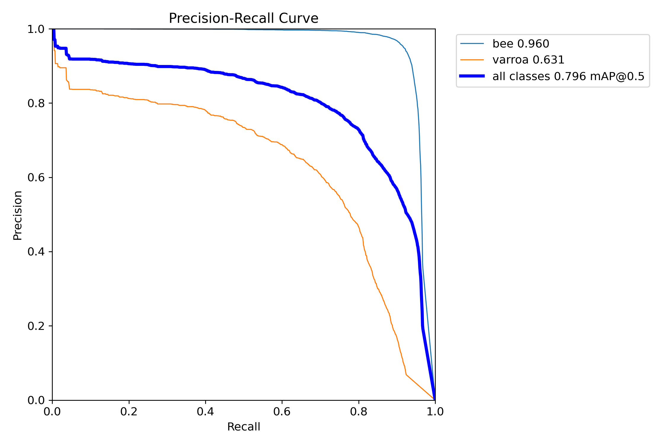
Precision-Recall Tradeoff
The PR Curve reveals the gap
between classes. Bee detection is near-perfect (0.96 mAP), while the Varroa curve (0.63 mAP) drops sharply —
the model struggles to maintain accuracy as it tries to find more mites.
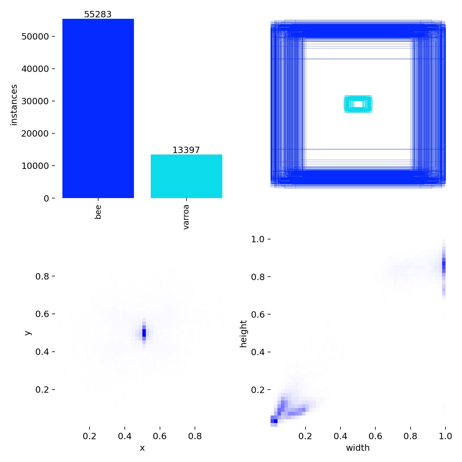
Class Imbalance & The P2 Plan
Labels.jpg confirms the ~4:1 bee-to-varroa class imbalance visible in the dataset. In object detection, this
can cause the model to favor the "easier" majority class (Bees) while neglecting the "harder" minority class
(Varroa).
Why P2? Because varroa mites are often less than 10 pixels wide. A P2 detection
head analyses at stride 4 (higher resolution) to ensure tiny features aren't lost in the feature
pyramid.
Figure 4: Spatial distribution and instance counts of Bee vs. Varroa labels.
Key Findings Across All Experiments
RT-DETR leads overall
RT-DETR achieves mAP50=0.9635 and mAP50-95=0.6406 — outperforming the best YOLOv8s run by
+0.018 and +0.033 respectively, with recall up +0.027.
The transformer architecture generalises better on classification without needing the cls=0.05 fix.
All runs still converging at epoch 200
Best epochs occur at 196–200 across every experiment. Extended training with early stopping is the clear next
step — particularly for RT-DETR, whose mAP50-95 curve shows no sign of plateauing.
cls=0.05 is the strongest single YOLO change
Reducing classification loss weight from 2.0 to 0.05 consistently improved mAP50-95 and eliminated the rising
val cls loss seen in cls=2.0 runs after epoch 50 — a clear sign of overfitting on classification.
Mixup augmentation showed no consistent benefit across either dataset scale.
2 datasets outperform 124 datasets
All 2-dataset runs score ~0.94+ mAP50 vs ~0.86–0.89 for 124-dataset runs. The gap points to quality
differences or distribution mismatch in the extended dataset pool — consistent with the findings from the
Debug Saga.
Training Curves
All 7 runs plotted over 200 epochs. Hover for per-run values.
Experiment Legend
mAP50 — Validation
mAP50-95 — Validation
Val Classification Loss
Val Box / GIoU Loss
Note on Val Box / GIoU Loss
RT-DETR uses GIoU loss for bounding box regression while YOLOv8s uses CIoU-based box loss.
The two losses operate on different scales (~0.28–0.41 vs ~1.02–1.24) and are not directly
comparable — treat them as independent convergence indicators per architecture.
📌 Context: Step 3 confirmed RT-DETR and cls=0.05 as promising directions (200ep each). This step
pushes further — extending YOLOv8s to 400/1000/2000 epochs, scaling up to YOLOv8L, and running RT-DETR-L to 1000
epochs with full training data captured.
At 1000 epochs, YOLOv8L surpasses all previous runs on every metric. Most strikingly, background→varroa false
positives collapsed from 237 (YOLOv8s 2000ep) to just 98 — a 59% single-run
improvement and 79% reduction from the starting point. The larger model's extra capacity is clearly doing real
work on the hardest class.
Metric Charts
YOLOv8s 200ep
YOLOv8s 400ep
YOLOv8s 1000ep
YOLOv8s 2000ep
YOLOv8L 1000ep
RT-DETR-L 200ep
RT-DETR-L 1000ep
Loss Curves
Val DFL Loss — a recurring pattern
Both YOLOv8s 2000ep and YOLOv8L 1000ep show val DFL loss rising after an early minimum (~ep300 for L), while
train DFL continues declining. This appears to be a fundamental characteristic of this dataset with the YOLO
architecture — the model learns bounding box distributions on training images that don't perfectly generalise.
YOLOv8L shows the same signature but with much better overall metrics, suggesting the extra capacity
compensates via better feature learning elsewhere.
On every headline metric, YOLOv8L 1000ep beats RT-DETR 1000ep: mAP50 0.971 vs 0.964,
mAP50-95 0.831 vs 0.789, precision 0.979 vs 0.953, recall 0.950 vs 0.929. The convolutional architecture
with larger capacity outperforms the transformer on this dataset.
RT-DETR Beats YOLOv8L on BG→Varroa FP
RT-DETR 1000ep gets 171 BG→varroa false positives vs YOLOv8L's 98 — so it doesn't
beat the FP benchmark either. However this is a massive improvement from the 555 at 200ep, confirming it was
just undertrained then. The transformer attention is doing real work on the varroa/background distinction.
RT-DETR Has a Bee Miss Problem
The big red flag: 762 bees predicted as background (bee recall ~0.90 normalised).
YOLOv8L has essentially zero of this — bees are saturated across all YOLO runs. RT-DETR is trading bee
detection confidence for varroa sensitivity in a way YOLO never did. The val cls_loss also spikes hard after
ep820, suggesting the model started overfitting its classification head late in training.
Val Cls Loss Spike — Overfit Signal
Val cls_loss reached its minimum at epoch 820 (0.275) then rose sharply to 0.407 by
ep1000. This is the RT-DETR equivalent of the YOLO val DFL divergence — the classification head is
overfitting. Best mAP50 was actually at ep818 (0.969), suggesting the saved weights at that checkpoint would
be stronger than the final model.
mAP50-95 Still Rising at ep1000
Like YOLOv8L, RT-DETR's mAP50-95 was still climbing at epoch 1000 (best at ep999:
0.789). Box localisation is still improving even as classification starts to overfit. This is a consistent
pattern across both architectures on this dataset.
Production Candidate: YOLOv8L
YOLOv8L 1000ep is the clear winner: best mAP50, best mAP50-95, lowest FP, highest
precision and recall, no bee miss problem. The best checkpoint (ep783 weights) is the strongest model in the
series. RT-DETR would need architectural tuning or more data to close the gap.